High-precision reference template for calibrating gear measuring instruments (4)
Evaluation of calibration results
The diameter of the probe probe, the mounting accuracy of the DBA on the detector, and the adjustment accuracy of the base circle radius all have a great influence on the peak point A of the hump curve.
The line connecting the center of the detection ball to the center of the probe for measuring peak point A is not tangent to the base circle, which is why the measured peak point A value is particularly sensitive to the position size. On the other hand, this feature is very useful for the curve fitting of the TCB to the MCB and for finding the cause of the error of the calibration detector.
The position of the valley bottom and the position of the peak point B are not greatly affected by the change of the parameters, and are quite stable. This is because at the valley V and peak B positions of the hump curve, the line connecting the center of the ball and the center of the probe is tangent to the base circle, that is, the points of the valley V and the peak B and the points on the involute are Corresponding point.
It is assumed that the measurement is normally completed and the DCE curve is obtained. In order to evaluate the DCE to calibrate the accuracy of the detector, we should determine the evaluation range of the output curve, namely the FK segments in Figures 2 and 5. The points F and K correspond to the quality control range of the involute profile at the proximal root and the top of the tooth on the line of action, respectively.
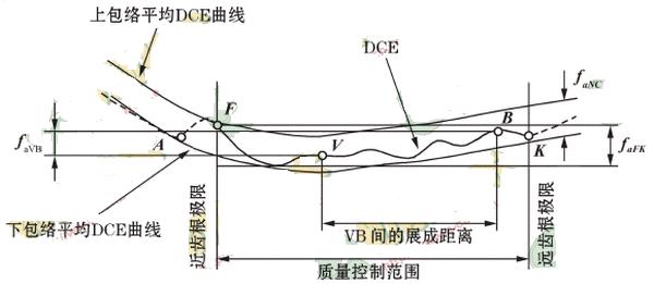
Figure 5 Some definitions that may be required to calibrate the accuracy of the involute detector using a spherical template
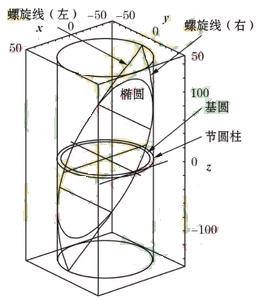
Figure 6 Principle of wedge pattern lead calibration
There are two different assessment methods:
Method 1: Calculate the TCB as a function of the nominal parameter value given by the technical conditions, then calculate the DCE by the curve fitting of the TCB to the MCB, calculate the sum of the squares of the difference between the MCB and the TCB, and divide the square root of the sum by the sample. Decreasing the number by one gives the standard deviation of the curve fit, which is a quality indicator of the calibrated detector. The DCE curve in Figure 2 shows an example of this evaluation with a standard deviation of 0.871 μm. Figure 5 shows a DCE curve. Points V and B are marked within the quality control range (ie, within the evaluation range), corresponding to the valley point and the peak point B of the hump curve, respectively. Considering the stability of V and B to determine the deviation value, the y difference faVB between these two points can be used as another quality indicator of the detector. The ratio of faVB to the developed length VB corresponds to the pressure angle error that the detector will produce. The DCE amplitude faFK over the entire length of the evaluation range FK can also be used as another quality indicator for the detector. After obtaining a smooth polynomial curve as the average curve of the DCE, we move the smooth average curve up and down to include the entire DCE curve, and the y difference between the upper and lower positions of the average curve tangent to the DCE curve is faNC It can also be used as another quality indicator for the detector. The faNC value corresponds to the wave noise of the detector and is included in the measurement results.
Method 2: Obtain the flattest DCE curve by correcting the nominal parameter values ​​of the TCB curve (such as magnification ratio, base circle radius, probe position error, etc.). The flat DCE curve 4 in Figure 3 shows an example of this rating with a standard deviation of the curve fit of about 0.094 μm. If the corrected DCE curve is sufficiently flat, the amount of change in each parameter when the curve is corrected corresponds to each error term of the calibrated detector. In this case, the standard deviation of the curve fit indicates the reliability of the measurement. The expected error of the detector is as follows: the base circle radius adjustment error: about 0.001 mm when rb=43.750mm; the probe magnification ratio error: about -6.6% (the negative sign indicates that the output value is less than the true value).
In Figure 2, the corrected curve 4 is fairly flat. We can determine that the quality of the detector is very good, but the amplification ratio of the instrument needs to be corrected.
If the corrected DCE curve is not flat enough, then the measurement results are worth exploring: the amount of parameter change at the time of correction corresponds to the possible error term of the detector. In addition, faVB, faFK and faNC should be considered at the same time.
Previous page next page